Note
This technote is not yet published.
Summary of the validation testing performed on the Data Preview 0.2 processing.
1 Introduction
To be written.
2 Single Frame Processing: Astrometry V&V
A detailed investigation on the quality of the astrometric calibration of the Single Frame Processing (SFP) stage of the Rubin Observatory LSST Science Pipelines was performed on the PREOPS-850 Jira ticket. The analysis is based on the processing of test datasets with the aim of asserting the fidelity of the Science Pipelines before kicking off the SFP of the full DP0.2 dataset. A brief summary of the findings is provided here. Please refer to that ticket for further plots and details. Note that this investigation does not include any measurement or assessment of the “Key Performance Metrics” defined in DOCUMENT?, which largely involve the inter-visit repeatablility statistics. These will be computed using the faro package and reported ELSEWHERE.
The executive summary is that, as of the v23_0_0_rc3 tag of the LSST Science Pipelines, the DP0.2 V&V team asserts that the quality of the astrometric calibration per detector/visit for SFP meets expectations for the SFP of the full DP0.2 dataset to proceed.
The following subsections describe a few of the “metrics” used to qualify the above statement.
2.1 Mean On-Sky Distance: Reference vs. Source
An examination of the distrubutions of the mean on-sky distance (in arcsec) between matched source and reference objects post-fit, for the entire test sample as well as per-band.
Of note was the identification of two detectors as astrometric “outliers”, in that they had mean on-sky distances well outside the range covered by the rest of the sample. We very much want to avoid having detectors with bad calibrations polluting the coadds, so an action was taken to add a threshold on this metric above which the astrometric fit is deemed a “failure”, keeping calibrated visit-level exposures from consideration in coaddition. Following the implementation, the two outliers did indeed disappear from the outputs with no other changes observed (as desired). The resulting distribution of the mean on-sky distance has a maximum value of ~0.02 arcsec (which may seem almost too good to anyone familiar with even the highest-quality real datat, but because of the nature of the simulations and the “perfectness” of the reference catalog, this value does make sense in this context).
The following plots show the before (two outliers observed) and after (two outliers now gone):
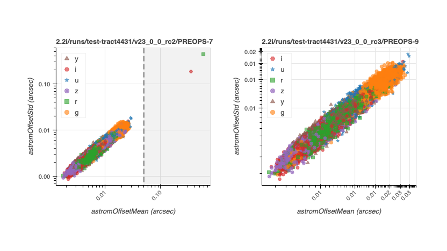
Standard deviation versus mean on-sky distance between reference and matched sources for SFP astrometric calibration. Left: pre-thresholding. Right: post-thresholding.
2.2 WCS scatter as a funtion of position on the focal plane
The following plots the mean astrometry distance as a function of position in the focal plane:

Distribution of the mean astrometry distance as a function of position in the focal plane. Each visit/detector gets a single point and, for visualization purposes, the position each point is staggered within the detector boundaries.
No trend with position on the focal plane is observed.
The investigation on the ticket went a bit deeper into issues related to the camera geometry currently implemented for LSSTCam-imSim by looking at the difference between the raw and SFP-calibrated WCSs. It is known that the simulations include a radial distortion and this does turn up in analysi (vizualized with quiver plots of vectors from raw-to-SFM-calibrated detector positions in focal plane coordinates). Also apparent is an effect from the differential chromatic refraction that is included in the models (and not yet corrected for in the pipelines, though work on this front is in progress). This is all good news as it indicates that the astrometric fitter is doing its job very well and, from another angle, there is good promise that we will be able to calibrate these effects out with future efforts (and this analysis will provide some validation of such calibrations).
Finally, the following is the version of the astrometry offset std vs. mean for the (now complete) full DP0.2 processing;
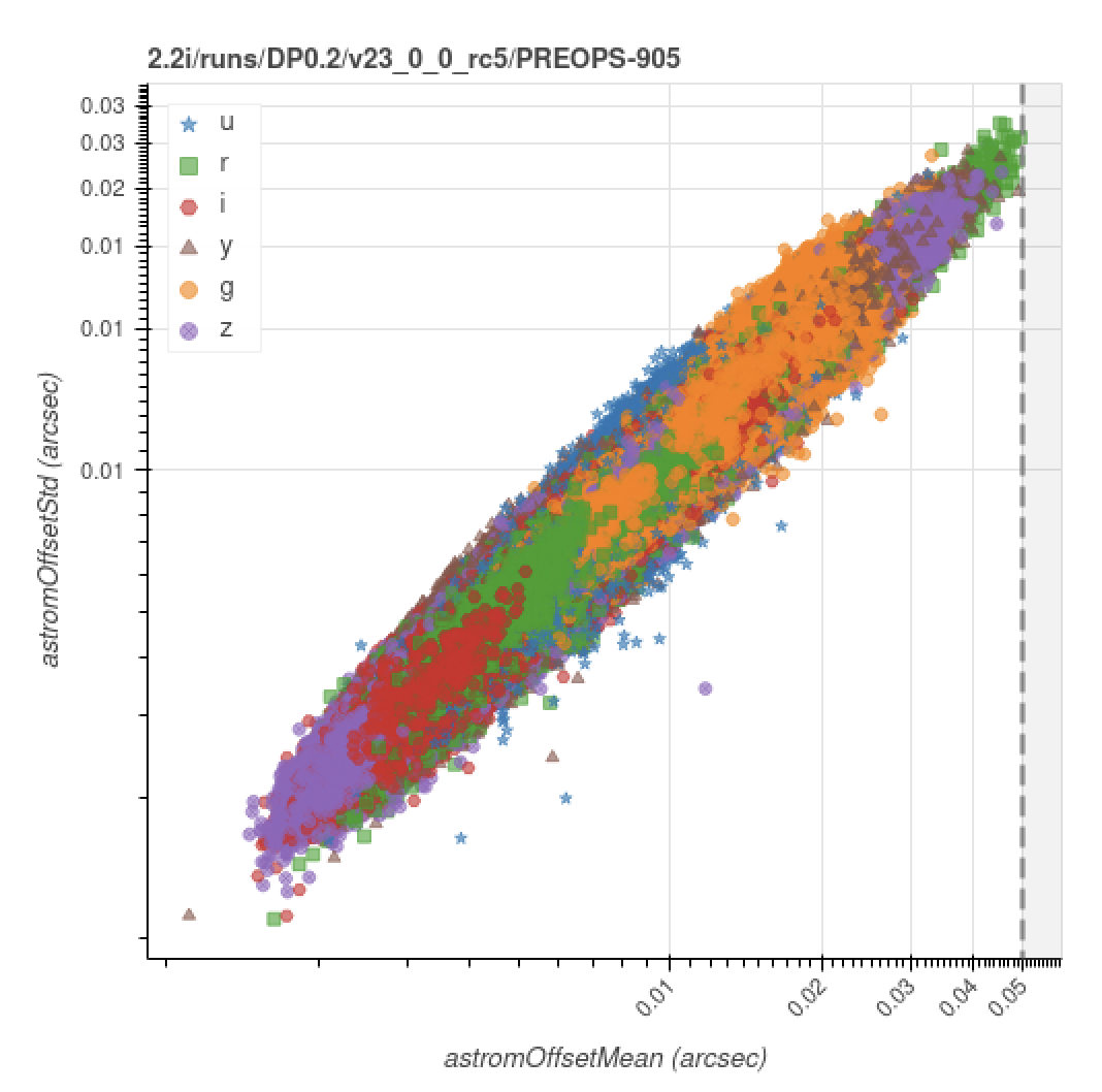
Standard deviation versus mean on-sky distance between reference and matched sources for SFP astrometric calibration for the full DP0.2 processing run (\(N_\mathrm{visit} = 19852\), \(N_\mathrm{detector} = 2804994\)).
Please refer to section-sfm-dp0p2-vv for further visualizations of the full DP0.2 SFP processing results.
3 Light curves from forced photometry
The test data for this investigation is three tracts of simulated data stored in the data-int cloud.
All datasets were processed through the Data Release Production pipeline using LSST Science Pipelines v23_0_0_rc2.
The data products analyzed here reside in two Butler collections: 2.2i/runs/test-med-1/v23_0_0_rc2/PREOPS-863 (tracts 3828 and 3829 with shallower depth, i.e., fewer visits) and 2.2i/runs/test-tract4431/v23_0_0_rc2/PREOPS-728 (tract 4431 with a five-year depth, i.e., more visits).
All datasets use the standard DC2 skymap with the LSSTCam-imSim instrument and contain patches from 0 to 48.
However, it is important to note that not every patch necessarily contains visits that span the full depth of all the observations.
To inspect the quality of forced photometry in these data, we use the Butler to load two dataset types, forced source tables (forcedSourceTable) and CCD visit tables (ccdVisitTable).
The former contains one row per image source, with information like bandpass and PSF flux measurements.
The latter contains one row per detector-visit pair, and we use this to retrieve the time of observation for each forced source.
A sample light curve for a single object is in Figure 4. The term “object” refers to an astrophysical object, while a “source” refers to a single detection or measurement of that astrophysical object, typically on a processed visit image. The photometry performed here is “forced” because it measures flux at a predetermined location where the object is expected to be rather than measuring the location of a PSF peak.

Figure 4 Light curve for one object in DC2 tract 3828. The y-axis shows psfFlux with psfFluxErr error bars, in units of nJy. Point colors correspond to bands, and dashed lines are to guide the eye.
We did experiment with computing two variability metrics: the weighted coefficient of variation and the median absolute deviation. The former uses the flux error whereas the latter relies on median statistics to quantify variability.
As an example, we computed that the light curve above has the following properties:
| band | N obs | weighted coeff var | median abs dev |
|---|---|---|---|
| u | 9 | 0.566 | 159.88 |
| g | 9 | 0.171 | 34.92 |
| r | 19 | 0.449 | 96.18 |
| i | 26 | 0.682 | 200.22 |
| z | 9 | 0.503 | 295.28 |
| y | 14 | 1.124 | 367.64 |
Each is a per-object metric rather than a per-source metric, and therefore does not appear in the forced source table. This kind of analysis and subsequent plots should be written as a Pipeline Task since it is not feasible to run for more than a few thousand objects at a time within an analysis notebook.
In Section 3.1 Big data, big memory challenges, we show some aggregate results from inspecting fluxes in a handful of patches in the three tracts described above. In Section 3.2 A (very small) sampling of light curves, we describe a closer look at a very small subset of object light curves. Finally, we discuss the additional tooling and analysis work necessary to more fully vet forced photometry light curve data products.
3.1 Big data, big memory challenges
The forced source tables exist on a per-patch basis. While each tract has 49 patches of data, loading even the bare minimum of columns into memory (via pandas for analsis in a jupyter notebook, for instance) is prohibitive for more than a few patches at a time. As a result, the most data we aggregated at one time is from 5 patches for one of the shallower tracts. Distributions of the forced PSF flux for all sources in patches 0–4 of tract 3898 are shown in Figure 5. We examined a single patch’s forced difference flux for all sources as well, shown in Figure 6. Nothing unusual is apparent in these plots, but they also do not provide the kind of granular object-level light curved vetting desired.

Figure 5 Forced flux distributions by band for all sources in tract 3828, patches 0–4.

Figure 6 Forced flux distributions by band on the difference images for all sources in tract 3828, patch 47. Because most detected sources are not also difference imaging sources, most have a flux at or near zero.
The memory problem is particularly pronounced when creating and examining light curves. For example, it is straightforward to write down metrics one may use to characterize light curve variability, or to search by sky coordinate for a known variable object of interest. It is much more challenging to meaningfully examine light curves for a representative sample of objects.
3.2 A (very small) sampling of light curves
We created a large pandas dataframe for a few patches of each tract by merging forced source table columns forcedSourceId (the index), band, psfFlux, psfFluxErr, and objectId with CCD visit table column expMidpt by merging on the shared column ccdVisitId.
We then identified all unique objects and plotted light curves for a subset of them.
Here we reproduce five light curves from each of three tracts. All y-axis values are force PSF fluxes in units of nJy.


3.2.3 Tract 4431 (deeper)


The deeper nature of tract 4431 is immediately apparent, as it has “observations” spanning from 2022 (ha) through 2027, whereas the shallower tracts 3828 and 3829 end in Q1 2023. Also apparent in most light curves is the larger scatter of y-band data points. In each Figure, the y-axis is auto-scaled to fit the data.
A couple of likely truly-variable astrophysically-interesting objects appear in the third and fifth plots shown for tract 3828. Noteable features include small error bars and significant flux changes over time.
Interestingly, some few flux measurements are less than zero, but they typically have large error bars that make them consistent with zero flux. This is probably mostly happening with fainter noise-dominated sources. It would be worthwhile to examine a cutout image of at least one epoch for each object’s light curve to get a better handle on this.
Overall, the light curves for all tracts look roughly as expected, with significant noise in the y-band. The y-band fluxes also tend to be brightest for all the objects plotted; it’s unclear if this is a real trend or just small number statistics. The process for selecting which light curves to plot could be improved by imposing a signal-to-noise or faint magnitude cutoff, as the handful of noise-dominated sources are probably very faint and not worth examining in detail.
In the future, we plan to turn the notebook analysis summarized here into a Pipeline Task that creates and persists light curve plots and relevant summary statistics on a per-object basis via the Butler. This will enable a more thorough variability analysis. In particular, it will enable us to investigate how accurately these metrics measure variability for known variable objects and better assess the performance of forced photometry in the Science Pipelines. We intend to use one or more variability metrics to identify which objects exhibit real astrophysical variability along with a high signal-to-noise ratio, because they are the ones we ought to examine in more detail to assessing pipeline performance.